해양 선박 분류를 위한 Gabor 기능 표현 및 딥 컨볼루션 신경망
Gabor Feature Representation and Deep Convolution Neural Network for Marine Vessel Classification
Article information
Trans Abstract
The Vessel Surveillance System (VSS), a crucial tool for fisheries monitoring, controlling, and surveillance, has been required to use for the reservation of the current depressed state of the world's fisheries by fisheries management agencies. An important issue in the vessel surveillance system is the classification of vessels. However, several factors, such as lighting, congestion, and sea state, will affect the vessel's appearance, making it more difficult to classify vessels. There are two main methods for conventional classifications of vessels: the traditional-based- characteristics method and the convolutional neural networks-used method. In this paper, we combine Gabor feature representation (GFR) and deep convolution neural network (DCNN) to classify vessels. Gabor filters in different directions and ratios are used to extract vessel characteristics to create a new image of vessels, which is DCNN's input. The visible and infrared spectrums (VAIS) dataset, the world's first publicly available dataset for paired infrared and visible vessel images, was used to validate the proposed method (GFR-DCNN). The numerical results showed that GFR-DCNN is more accurate than other methods.
1. Introduction
Maritime activities that affect economic and social development are important to human society, for example, shipping, trade, maritime security, and anti-illegal activities. In maritime surveillance, the correct classification of vessels is very important and significant for sea operations. Vessels classification is more difficult compared to other target identification problems, due to the large variation in observed perspective, illumination conditions, scale, and unorganized background image (Shi et al., 2019).
Deep learning-based and handcrafted feature-based methods are the two main available techniques for classifying marine vessels (Zhang et al., 2019). Also, global feature-based techniques and local feature-based techniques are two branches inside the handcrafted feature-based methods. In the past, low-level global geographic features assisted in ship classifications like geometry characteristics, including proportions, aspect ratio, and shape. However, the geometry cannot be used in complex cases. Some local features such as the position of the masts were found to be more discriminatory in ships classifications (Min and Dongping, 2005). Hierarchical multi-scale LBP (HMLBP) (Guo et al., 2010), which obtain local features, dramatically increase the performances of classification. Moreover, various feature frameworks, like the MSHOG feature-based task-driven vocabulary training (Lin et al., 2018), join both the global and local features. Thanks to the development of deep learning technology, many tasks of computer vision and image classification have achieved a lot of improvement. The deep learning approach gives more discriminative high-level visual features, compared with the handcrafted feature approach. These features fill in the existing gap between the hand-crafted feature description and the vessel image content. Among the deep-learning approach for ship classification, Shi et al. (2018) applied 2D discrete fractional Fourier transform (2D-DFrFT) and two-branch CNN to obtain features. 2D-DFrFT and LBP (CLBP), which extracted various traditional features, was used to get the high-level abstract features (Shi et al., 2019). Literature (Akilan et al., 2018) used Inception-V3, VGG-16, and AlexNet to obtain the image descriptions and normalizes various features to the identical feature space. The authors in (Zhang et al., 2015) used the VGG-16 CNN structure with the ImageNet database to extract features from the 15th layer. Literature (Khellal et al., 2018) used machine learning for getting the relationship of multi-color characteristics. Literature (Khellal et al., 2018) introduced a new method, ELM, detecting discriminative CNN features. Authors in (Shi et al., 2019) created a classification framework, ME-CNN, using a multi-feature ensemble. The deep learning based-method presents powerful feature extraction in comparison with the conventional methods.
Gabor filters have many advantages, and they get higher accuracy when compare with other feature extraction techniques such as Local Binary Pattern (LBP), Principal Component Analysis (PCA) (Allagwail et al., 2019). This work introduces the novel method for marine vessel classification using a deep learning approach base on the Gabor filter. We create a Gabor feature representation to extract the features of vessel images and apply a deep convolution neural network to classify these extracted features.
2. Gabor Feature Representation and Deep Convolution Neural Network
2.1 Gabor filter
The 2D Gabor filter, the core of Gabor filter-based feature extraction, will be created from the multiplication between an elliptical Gaussian and a sinusoidal plane wave (Kamarainen, 2010). A major and minor axis by γ and η control the sharpness of the filter. The filter response has a compact closed-form:
where ϕ is the rotation angle of both the Gaussian primary axis and the plane wave, fc is the center frequency of the filter, η is the sharpness along the secondary axis and γ is the sharpness along the primary axis.
Gabor bank or Gabor features are created from replies of Gabor filters in equation (1) by applying multiple filters on various frequencies fs and orientations ϕv. Frequency, in this situation, agrees to scale data and is thus described by:
where fmax is the maximum frequency wanted, fs is the sth frequency, and k > 1 is the frequency scaling element. The filter orientations are described by:
where V is the entire amount of orientations and ϕv is the vth orientation.
Exponential spacing and orientations from linear spacing determine scales of a Gabor filter. Valid values of orientation vary from 0 to 2π. The bands of Gabor filters rotate with a variety of orientation values.
2.2 Gabor feature representation
Gabor wavelet-based algorithms have the advantage of recognizing ship images including different proportions, luminance, and directions. Fig. 1 shows the manner of forming a Gabor feature representation for the input image. The first row is the original image; the second row is the various Gabor filters; the third row is the responses with the Gabor filters; the last row is the final Gabor feature representation. We use different Gabor filters with k = 64 scales and M = 64 orientations and apply Inverse Fast Fourier Transform, Fast Fourier Transform, to speed up the computational convolution process. Both Gabor wavelets in the third row and the image in the first row are transformed to the frequency domain using FFT then their convolution is converted back to the spatial domain using IFFT. This spatial domain value is then used to create the final Gabor feature representation, as shown in the last row.

The manner of forming a Gabor feature representation
2.3 Deep convolution neural network
In the proposed method, derived from AlextNet, we did some modifications to the structure of DCNN. Firstly, we reduced the total convolution layers from five to four. The proposed network has four convolution blocks, while the Alexnet has two convolution blocks and three convolution layers. The layers in each convolution block are the convolution layer (or group convolution layer), ReLu layer, cross normalization layer (CN), and max-pooling layer, respectively. Secondly, the dropout layer, which can decrease the over-fitting, is joined to the network before the fully connected layer. Fig. 2 presents the comparison of the proposed deep convolution neural network and Alexnet structure.

The comparison of the proposed deep convolution neural network and Alexnet
The proposed deep convolution neural network applies one convolutional layer and three group convolution layers. The kernels for four convolution layers are 96 kernels of size 11×11×3, 192 kernels of size 7x7, 384 kernels of size 5×5, and 192 kernels of size 3×3, respectively. The stride is 4×4 for the first convolution layer and 2x2 for other group convolution layers. The structure creates the trainable feature maps, which are passed to fully connected layers. The output classification layer accepts the classification probabilities, are defined by the softmax layer. These classification probabilities in the softmax layer make categories of six classes.
3. Dataset and Experiment Result
3.1 Dataset
We employ the VAIS dataset (Zhang et al., 2015) in our evaluation. VAIS database, which was the earliest openly obtainable database shown at the CVPR 2015, includes both infrared and visible vessel images.
The dataset consists of a total of 2865 images, including 1623 visible and 1242 infrared images. We resize every vessel image to size 227 × 227 employing bicubic interpolation. There are six coarse-grained classes in the dataset, namely medium passenger, medium-other, merchant, sailing, small boats, and tugboats. The number of samples in each class is highly unbalanced, which raises the challenge of classification. The class number of the VAIS dataset in this work is given in Table 1. We use only the visible images for the comparison with other methods. As seen in Table 1, some classes have 140 images, while other classes have 412 images in the training set. Fig. 3 shows some visible samples from each class in the dataset. The various factors, including the size of ships, the uneven illumination, and the environment set a high demand for the features classification and are complicated.

The testing and training number in the VAIS dataset.
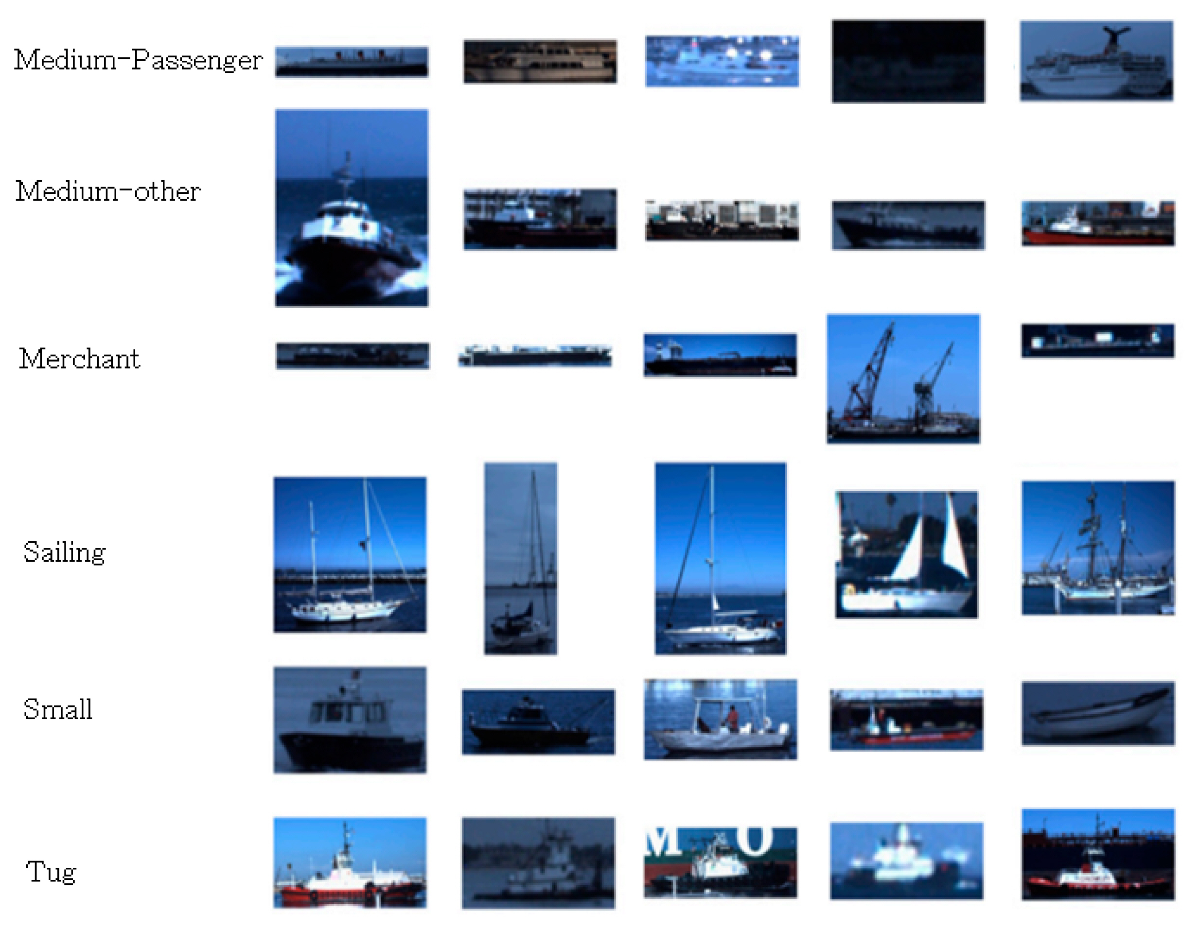
Some visible in the VAIS database
3.2 Experiment result
We compare the GFR-DCNN with other approaches, and the outcomes are presented in Table 2. The experimental conditions are similar in all approaches. Table 2 shows not only the deep learning in literature but also the conventional methods (HOG + SVM, LBP + SVM), SRDA, SFLPP, and the proposed GFR-DCNN gained the best accuracy.

The comparison of various method base on the VAIS database.
The GFR-DCNN enhances results against the conventional classification methods due to the combination of the Gabor filter for feature extraction and DCNN for classification. In most cases, both GFR and DCNN contribute to higher precision. For example, GFR-DCNN generates higher accuracy of 11.33% compared with the LBP+SVM method (Zhang et al., 2019). In this situation, GFR exceeds LBP, and DCNN surpasses SVM in the classification task.
The only case of the Gnostic Field + CNN method (Zhang et al., 2015), in which only GFR is more precise. Reference (Zhang et al., 2015) uses VGG16 as the CNN backbone, which outperforms in classification tasks compared to the AlexNet (Rangarajan et al., 2018). In this case, GFR is more accurate than Gnostic Field, and GFR-DCNN gets higher precision of 6.6% in comparison with the Gnostic Field + CNN method.
Table 3 displays the confusion matrix, which provides a precision of 87.60%. The class “medium other ships” obtained a high accuracy of 98.0% (predict right 194 MOS over the total of 198). Twenty-one images of merchant ships are wrong predicted as tugboats, which causes the most confusion.

The confusion matrix for multi-classification on the VAIS database.
4. Conclusion
Vessel classification is an essential topic in computer vision. Many researchers have researched this subject in various ways concerning many applications, which include Vessel Surveillance System, Automatic Identification System. This paper presents an application of deep learning and Gabor filters on vessel classification. Gabor filters in different directions and ratios are used to extract vessel characteristics to create a new image of vessels, which is DCNN's input. Our method could improve classification accuracy by 15.73%, compared with the other approaches. Further research is that the proposed GFR-DCNN will be integrated with the Automatic Identification System (Kim et al., 2016) to surveil the vessel. In addition, we will compare the proposed method with other approaches on the Korean ship dataset established by DB of National Information society agency (NIA, https://www.nia.or.kr/site/nia_kor/main.do).
Acknowledgements
This research was supported by the Basic Science Research Program through the National Research Foundation of Korea (NRF) funded by the Ministry of Education (2020R1I1A306659411, 2020R1F1A1069124), and Ministry of Trade, Industry and Energy for its financial support of the project titled “the establishment of advanced marine industry open laboratory and development of realistic convergence content”.
Notes
Funding
This research was funded by the Brain Korea 21 project (BK21).