In this study, the Finite Volume Coastal Ocean Model (FVCOM) was used to simulate the seawater circulation (Chen et al., 2006). The governing equation in the FVCOM model consists of the momentum equations (Eqs. 1~3), the continuity equation (Eq. 4), temperature (Eq. 5), salinity (Eq. 6), and density (Eq. 7):

where x, y, and z are the east, north, and vertical axes in the Cartesian coordinates system; u, v, and w are the x, y, and z velocity components; T is the temperature; S is the salinity; p is the density; P is the pressure; f is the Coriolis parameter; g is the gravitational acceleration; K_m is the vertical eddy viscosity coefficient; and K_h is the thermal vertical eddy diffusion coefficient. F_u, F_v, F_t, and F_s represent the horizontal momentum, thermal and salt diffusion terms, respectively. The total water column depth is D =H+ζ, where H is the depth and ζ is the height of the free surface (relative to z =0).

Vertical eddy mixing is calculated either by Mellor and Yamada level 2.5 (Mellor and Yamada, 1982) or the k −ɛ turbulence closure schemes (Rudi, 1987). The horizontal eddy viscosity and diffusion are calculated by the Smagorinsky's parameter (Smagorinsky, 1963). A σ transformation in the vertical axis is used to convert irregular bottom topography into a regular computational domain.

FVCOM subdivides the horizontal computational domain into a set of non overlapping unstructured triangular grid. An individual triangle is composed of three nodes, a centroid and three edges. The horizontal velocity components (u, v) are located at the triangle centroids and the vertical velocity as well as all scalar variables (temperature, salinity, etc.) are placed at the nodes. More about FVCOM is described in detail in Chen et al. (2006) and model validations as well as comparisons with other numerical models can be found in Chen et al. (2007) and Huang et al. (2008).

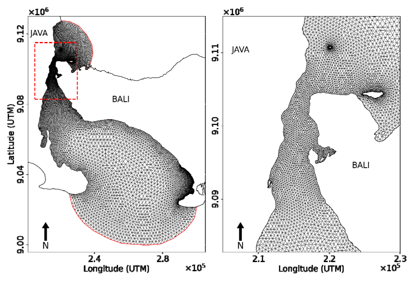
The triangular unstructured grid numerical model domain is shown in Fig. 2. Two open boundaries are located on the top and bottom of the domain (solid red line) while the close boundary is the coastline of Bali and East Java. The horizontal resolution (dx) in FVCOM is defined by the length of an individual triangle edge. In this study, the minimum and maximum horizontal resolutions were 50 m and 500 m, respectively. Small size grids were used at the narrow strait as shown by the intersect image in Fig. 2. In the vertical layer, the uniform layers with the 2nd σ layer were applied in this numerical simulation.

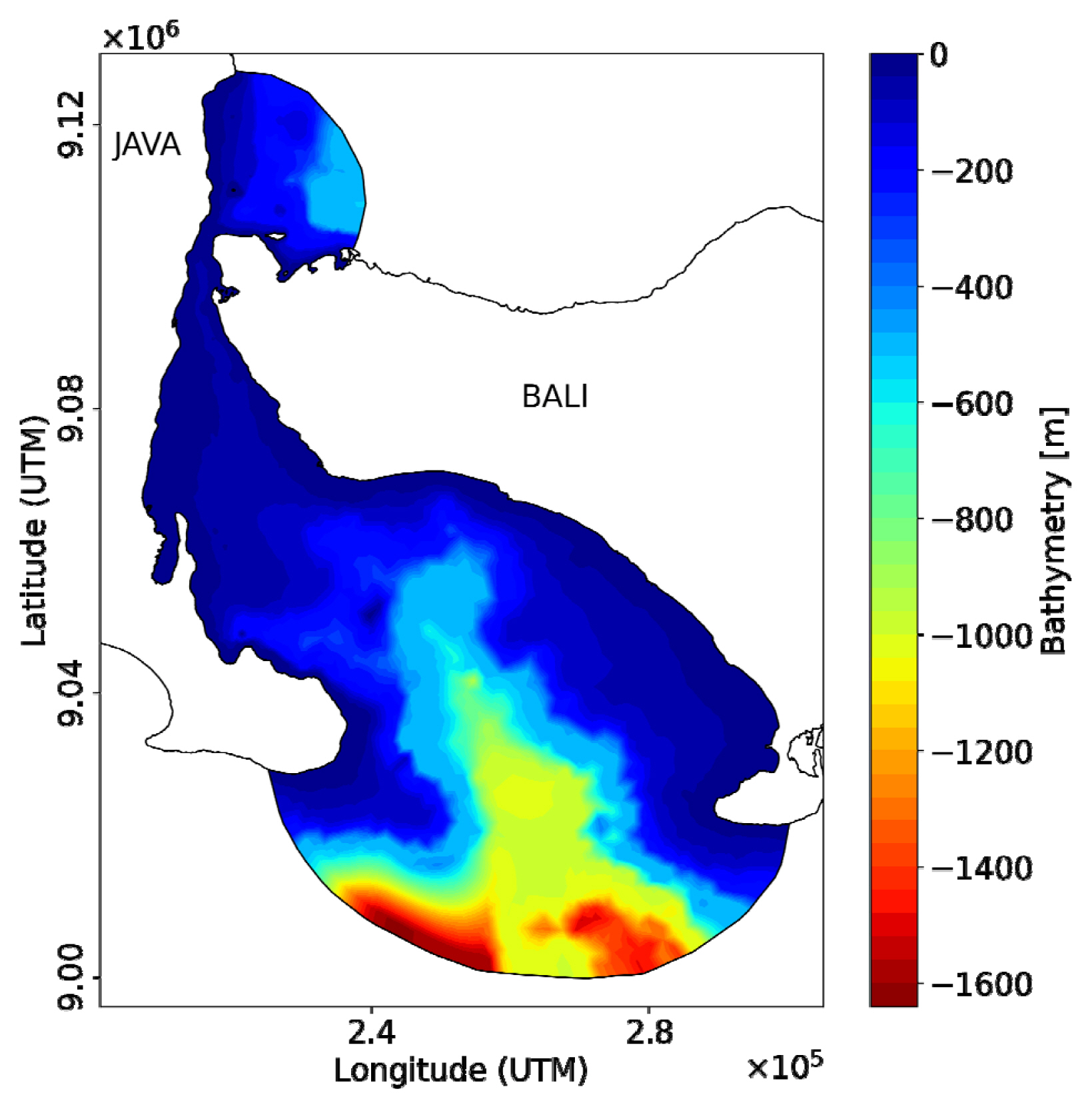
Fig. 3 shows the bathymetry map of Bali Strait obtained from Hydro-Oceanography Division, Indonesian Navy (DISHIDROS-TNI AL). Bali Strait is shallow in the middle of the narrow strait and steep at south of the strait, and directly faces to the Indian Ocean.

In this study, model inputs in the open boundary were tide elevations using 4 tidal components, S₂, M₂, K₁, and O₁. These tidal components were obtained from the tide elevation data by the Ocean Research Institute (ORI), University of Tokyo (ORI-Tide) (Matsumoto et al. 1995). Temperature and salinity were set to be constant. The 5 year-averaged wind data obtained from the European Center for Medium-Range Weather Forecast (ECMWF) were used as the meteorological wind conditions. The vertical eddy viscosity and the vertical thermal diffusion coefficients were calculated using modified Mellor-Yamada level 2.5 (MY-2.5) turbulence closure model (Galperin et al., 1988). The horizontal diffusion coefficients were calculated using the Smagorinsky eddy parameterization method (Chen et al., 2003). The simulation was carried out for 30 days with time step of 1 second. The initial setup conditions are summarized in Table 1.

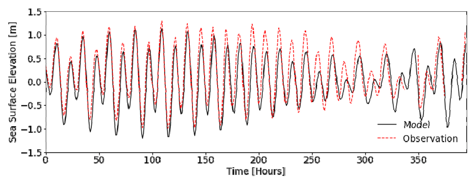
Sea surface elevations obtained from numerical simulation using FVCOM were compared with observation data obtained from the 1 hour tide-gauge time series measured at the Pengambengan Station (114°34′24.89″ East and 8°23′11.47″ South), which belongs to the Institute for Marine Research and Observation, under the Ministry of Marine Affairs and Fisheries of Indonesia. The time series of sea surface elevation from the numerical simulation and observation are shown in Fig. 4. The comparison shows that the numerical model is able to simulate the elevation of sea water in Bali strait.

For the quantitative validation, the root mean square error (RMSE) of seawater surface elevation obtained from the numerical simulation and observation was calculated as follows:

where x_o and x_m a re the value of the observations and model respectively and n is the total data. The RMSE is 0.086 m, which indicates a good agreement between the simulation and observation.

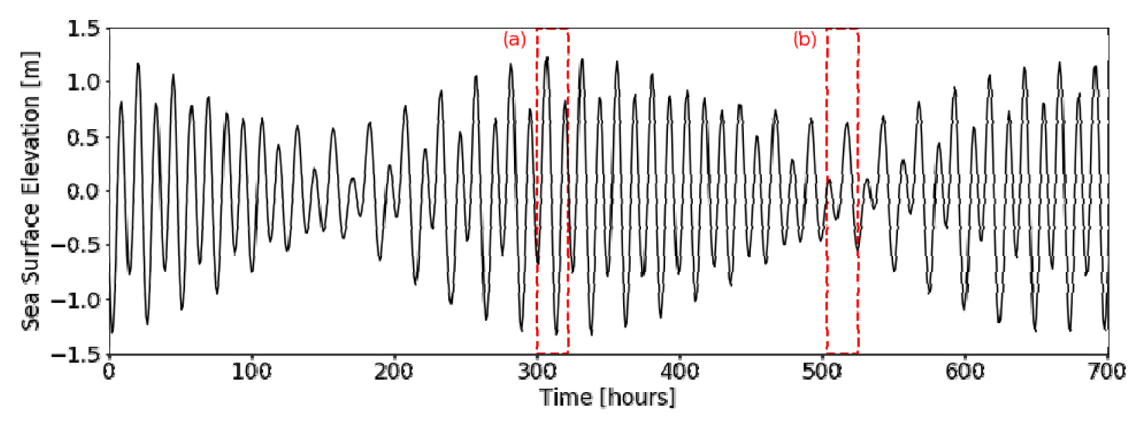
Fig. 5 shows a time series of seawater surface elevation obtained from the simulation. From the 30 days simulation, two spring tides and two neap tides are found. The spring tide (Fig. 5a) is the condition when the largest range of water surface elevation occurs while the neap tide (Fig. 5b) is the opposite condition. Moreover, two tides per day with a different range were occurred in Bali Strait. This indicates that Bali Strait has a mixed tide cycle or mixed semi-diurnal tide.

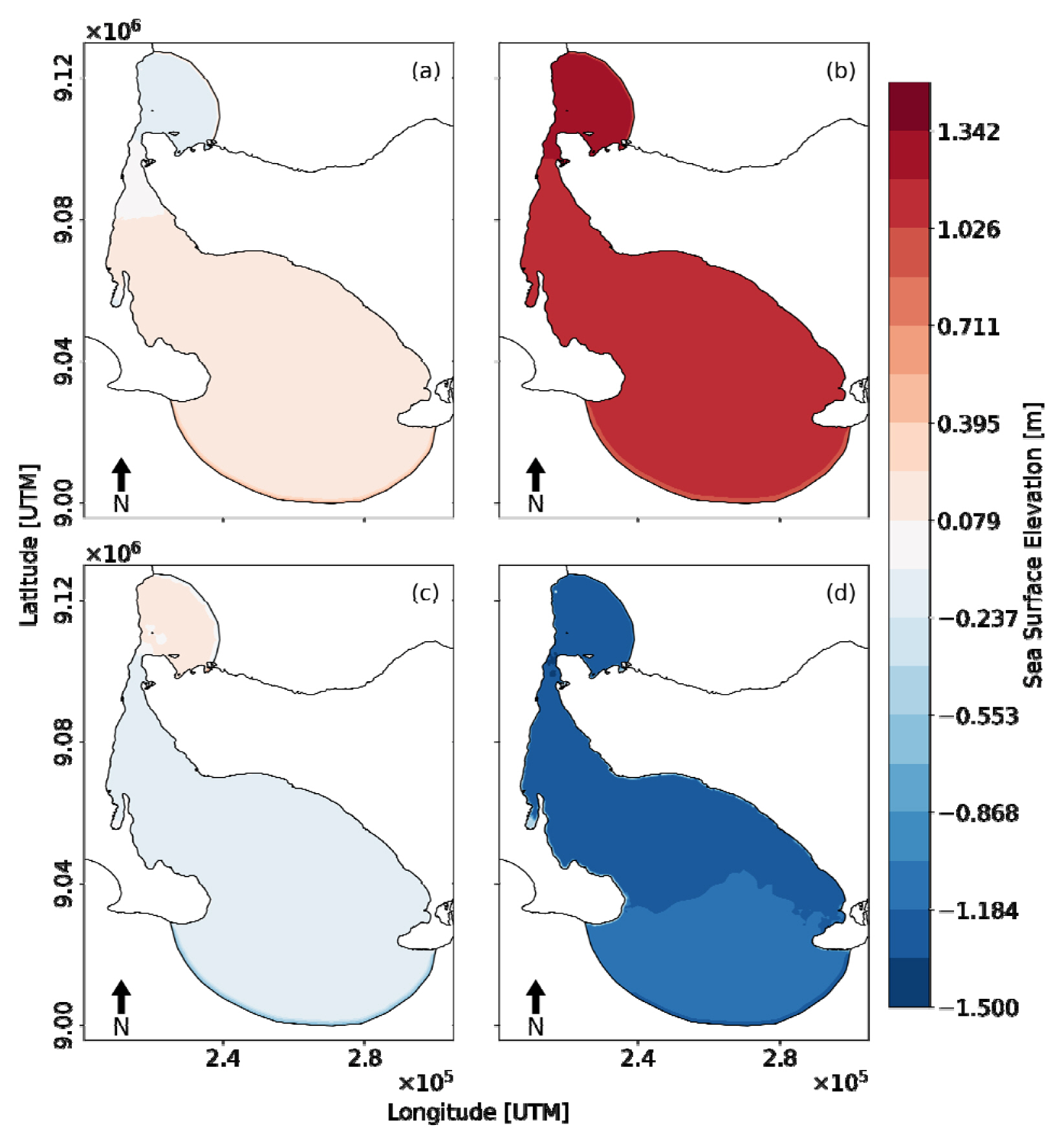
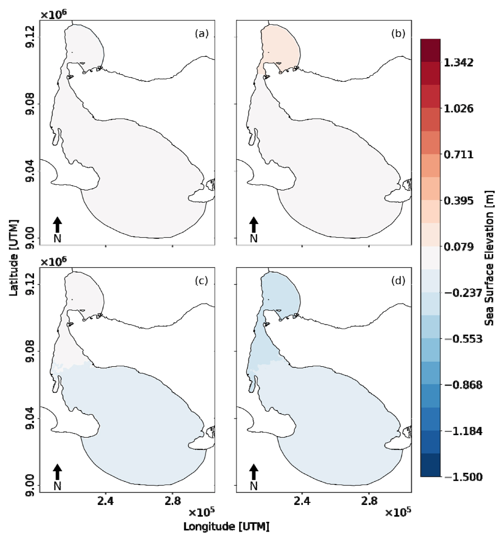
The spatial distributions of sea surface elevation during the spring tide and the neap tide are shown in Figs. 6 and 7, respectively. The four tide conditions consisting of flood tide, high tide, ebb tide and low tide were analyzed. The flood tide is the rising process from low water to high water. The high tide is the highest water elevation in one oscillation process. The ebb tide is the falling process from high water to low water. The low tide is the lowest water elevation in one oscillation.

Fig. 6a shows that the sea surface during the flood tide is higher in Indian Ocean than in Bali Sea. This condition leads to the water moving from Indian Ocean to the Bali Sea through the narrow strait between Bali and East Java until it reaches the high tide condition (Fig. 6b). The seawater then moves back to the Indian Ocean during ebb tide (Fig. 6c) until it reaches the low tide condition (Fig. 6d). The similar pattern of seawater movement is also found during the neap tide condition as shown in Fig. 7.

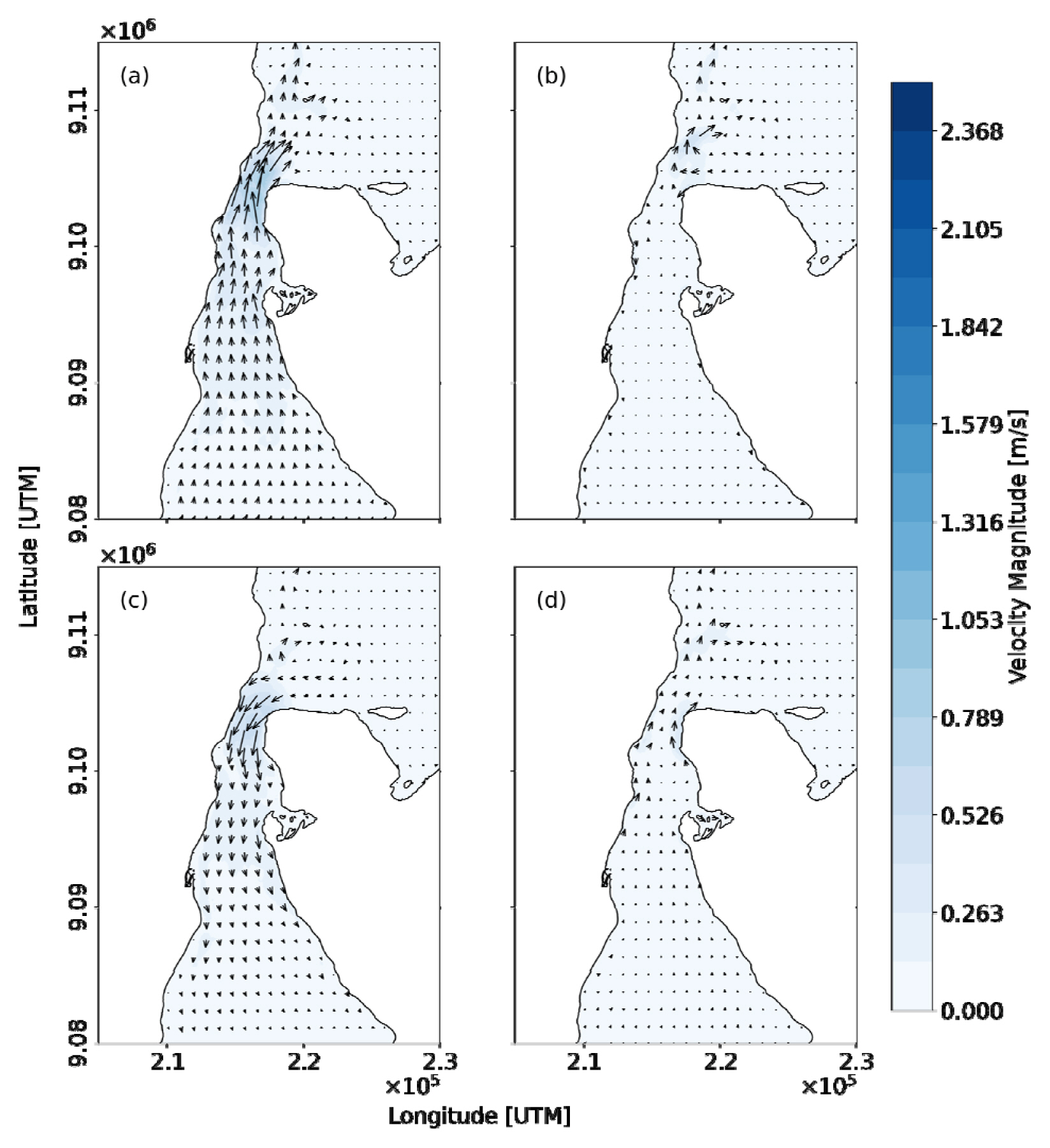
Tidal current on the seawater surface during the spring tide and neap tide conditions were analyzed and the results are shown in Figs. 8 and 9, respectively. Similar to the analysis in seawater surface elevation, the tidal current was analyzed during the flood, high, ebb and low tide conditions. The analyzed of tidal current focused on the narrow strait shows the highest velocity magnitude in this area.

During the spring tide condition, the seawater moves to the top of the narrow strait with the maximum velocity magnitude of 1.69 m/s (Fig. 8 a). This current then decreases to the maximum velocity magnitude of 0.85 m/s as the tide reaches the high tide condition (Fig. 8b). The seawater then rushes back to the Indian Ocean during the ebb tide with the maximum velocity magnitude of 2.25 m/s (Fig. 8c) until it reaches the low tide condition (Fig. 8d) with the maximum velocity of 0.8 m/s. During the high and low tide conditions, an eddy is observed on the top of the narrow strait. The similar pattern is also observed during the neap tide condition as shown in Fig. 9 while there is no eddy formed during the neap tide condition. The maximum current velocity magnitude is 0.91 m/s, which occurres during the flood tide in the neap tide conditions (Fig. 9a).